RaBitQ in Zvec: Quantization Principles, Index Design, and Benchmarks
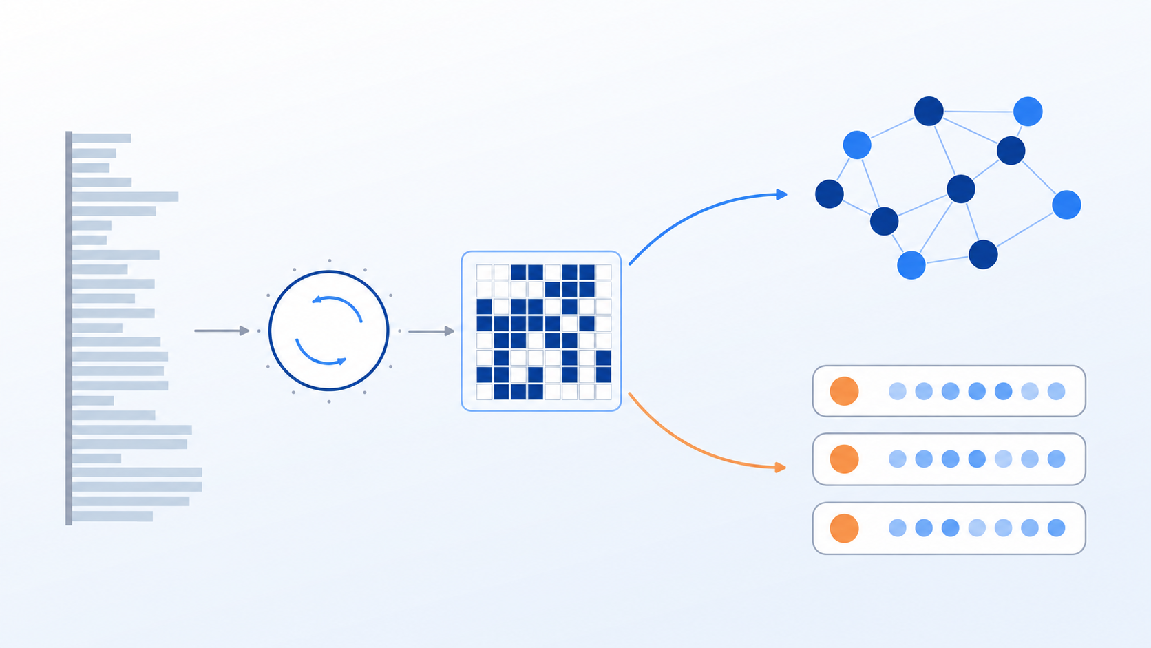
Abstract: Zvec now includes two native vector indexes, HNSW-RaBitQ and IVF-RaBitQ, with
total_bitscontrolling the tradeoff between compression and recall. In benchmarks on the same machine with 8 threads at matched Recall@10, HNSW-RaBitQ with 1-bit quantization and reranking delivers 11.0×–12.6× the throughput of Elasticsearch 8.18.8 BBQ on GIST-1M and 5.9×–16.0× on Cohere-1M. IVF-RaBitQ with 7-bit quantization delivers 3.2×–4.8× the throughput of Faiss.
RaBitQ: Making Quantization Error Estimable
Vector quantization reduces the number of bits per vector, lowering storage, memory bandwidth, and distance computation costs. The tradeoff is information loss: approximate distances can change the ordering of candidates. This error generally becomes more pronounced at lower bit widths, ultimately reducing recall.
Compared with traditional methods such as PQ and scalar quantization, RaBitQ generally provides more accurate distance estimates under the same bit budget. It also provides an error range for those estimates. During a query, this range can be used to eliminate some uncompetitive candidates early.
Benchmarks
The tests use 8 physical cores on the same Alibaba Cloud instance and cover GIST-1M and Cohere-1M, each containing one million vectors. The full environment and supplementary results are in the appendix.
The HNSW comparison uses 1-bit quantization with reranking on original vectors; the IVF comparison uses 7-bit quantization throughout. All performance figures follow two conventions: throughput is compared at matched Recall@10, and disk usage is compared using complete index directories (both the Zvec database and ES retain the original FP32 vectors). Comparisons are valid only within the respective HNSW and IVF groups. The HNSW comparison measures end-to-end system performance: Zvec uses in-process calls, while Elasticsearch includes local HTTP, single-shard scheduling, and coordination overhead. Their quantization and graph implementations also differ. The IVF comparison is closer to an algorithm-level comparison.
1-bit HNSW-RaBitQ vs Elasticsearch BBQ
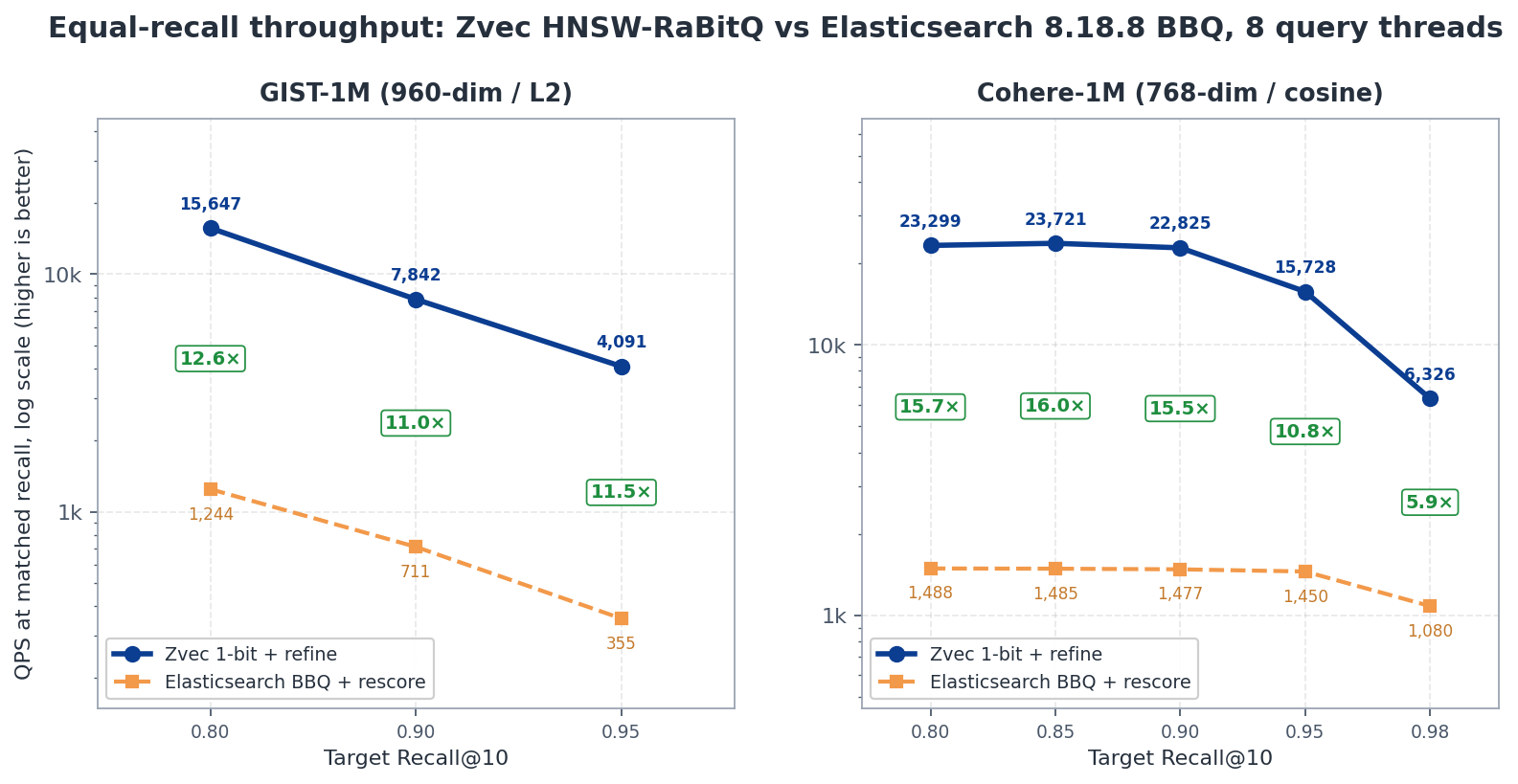
With 8 threads at matched recall, Zvec delivers 11.0×–12.6× the throughput of ES on GIST and 5.9×–16.0× on Cohere. As recall approaches its upper limit, more candidates require reranking, and the throughput advantage gradually narrows.
On GIST and Cohere, Zvec builds the database 3.04× and 2.32× as fast, respectively, with complete indexes that are 12% and 33% smaller. Both systems retain the original FP32 vectors, so directory sizes do not achieve the theoretical compression ratio of the quantized codes alone.
7-bit IVF-RaBitQ vs Faiss
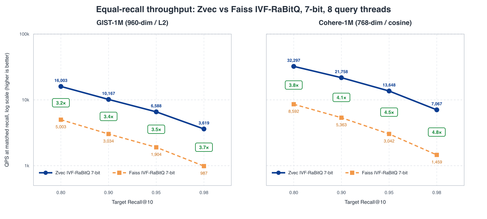
With 8 threads at matched recall, 7-bit Zvec delivers 3.2×–3.7× the throughput of Faiss on GIST-1M and 3.8×–4.8× on Cohere-1M. Recall is similar at the same nprobe value. Higher recall requires scanning more inverted lists, making Zvec's throughput advantage in batch scanning more pronounced.
Construction is the main cost: Zvec takes 1.52× as long on GIST and 1.04× as long on Cohere, with roughly 90% of the time spent on KMeans training. Its complete indexes are 6.5% and 24% smaller than Faiss, respectively.
Usage Examples
Both indexes use the standard Collection API. Select the corresponding index parameters in VectorSchema. Here is an HNSW-RaBitQ example:
import zvec
from zvec import (
    CollectionSchema,
    DataType,
    HnswRabitqIndexParam,
    HnswRabitqQueryParam,
    MetricType,
    OptimizeOption,
    Query,
    VectorSchema,
)

schema = CollectionSchema(
    name="hnsw_rabitq_demo",
    vectors=[
        VectorSchema(
            "embedding",
            DataType.VECTOR_FP32,
            dimension=768,
            index_param=HnswRabitqIndexParam(
                metric_type=MetricType.COSINE,
                total_bits=7,
                num_clusters=16,
                m=16,
                ef_construction=200,
            ),
        ),
    ],
)

collection = zvec.create_and_open(path="./hnsw_rabitq_demo", schema=schema)

# Document writes omitted.
# optimize() builds the accelerated HNSW-RaBitQ index.
collection.optimize(OptimizeOption())

results = collection.query(
    queries=Query(
        field_name="embedding",
        vector=query_embedding,
        param=HnswRabitqQueryParam(ef=300),
    ),
    topk=10,
)
IVF-RaBitQ follows the same workflow. Replace the index parameters with IvfRabitqIndexParam and use nprobe at query time to control the number of inverted lists to scan. optimize() performs training, construction, and persistence in sequence:
import zvec
from zvec import (
    CollectionSchema,
    DataType,
    IvfRabitqIndexParam,
    IvfRabitqQueryParam,
    MetricType,
    OptimizeOption,
    Query,
    VectorSchema,
)

schema = CollectionSchema(
    name="ivf_rabitq_demo",
    vectors=[
        VectorSchema(
            "embedding",
            DataType.VECTOR_FP32,
            dimension=768,
            index_param=IvfRabitqIndexParam(
                metric_type=MetricType.COSINE,
                nlist=1024,
                total_bits=7,
                sample_count=0,        # 0 means train on all available vectors
            ),
        ),
    ],
)

collection = zvec.create_and_open(path="./ivf_rabitq_demo", schema=schema)

# Bulk writes omitted.
collection.optimize(OptimizeOption())

results = collection.query(
    queries=Query(
        field_name="embedding",
        vector=query_embedding,
        param=IvfRabitqQueryParam(nprobe=20),
    ),
    topk=10,
)
The example uses nlist=1024 only to illustrate the API. In practice, choose this value based on the dataset size and distribution. An excessively large nlist on a small dataset produces many empty inverted lists.
For higher recall, in addition to tuning total_bits and nprobe, you can enable reranking with original vectors: first retrieve a set of candidates using RaBitQ, then read their FP32 vectors to compute exact distances.
query = Query(
    field_name="embedding",
    vector=query_embedding,
    param=IvfRabitqQueryParam(
        nprobe=20,
        is_using_refiner=True,
        scale_factor=10.0,   # candidate expansion ratio for rescoring, IVF-RaBitQ only
    ),
)
results = collection.query(queries=query, topk=10)
Keep two points in mind: scale_factor applies only to IVF-RaBitQ. HNSW-RaBitQ also supports is_using_refiner, but its initial candidate count is determined by max(topk, ef), so increasing ef is how you expand the candidate set.
Principles and Implementation
RaBitQ: Randomized Vector Quantization with a Theoretical Error Bound
RaBitQ[1], introduced by Jianyang Gao and Cheng Long at SIGMOD 2024, stands for Randomized Bit Quantization. Its central idea is to turn distance computation into inner-product estimation between unit vectors, then approximate vector directions using a randomly rotated regular codebook to keep quantization error low. At the same time, randomness concentrates a difficult-to-compute error term near zero in high-dimensional space, making it possible to estimate an upper bound on distance error.
Step 1: Turn a Distance Problem into a Direction Problem
Let the original data vector and query vector be oᵣ and qᵣ, and let the reference centroid be c. Normalize both vectors relative to the centroid to obtain unit directions o and q. For squared Euclidean distance:
||oᵣ-qᵣ||² = ||oᵣ-c||² + ||qᵣ-c||²
               - 2||oᵣ-c||||qᵣ-c||⟨o,q⟩
The distance from the data vector to the centroid can be stored during construction, and the distance from the query vector to the centroid needs to be computed only once. The only quantity that needs approximation is therefore the inner product of the unit directions, ⟨o,q⟩. In other words, the question RaBitQ needs to answer is: How close are these two directions?[4]
Step 2: Construct a Randomly Rotated 1-bit Codebook
RaBitQ starts with a hypercube inscribed in the unit sphere. Each vertex is a unit vector, with each coordinate taking either −1/√D or +1/√D:
C = {−1/√D, +1/√D}ᴰThis codebook has 2ᴰ vertices, but a vertex can be represented by D signs, requiring just 1 bit per dimension. RaBitQ then rotates the entire codebook using a random orthogonal matrix, randomizing its orientation relative to the data, and selects the nearest rotated codeword ō for each data direction. The theoretical description rotates the codebook; an equivalent implementation rotates the data and query vectors and encodes each coordinate by its sign. Orthogonal rotation preserves distances and inner products.[4]
Step 3: Build a Distance Estimator Using Concentration of Measure
Given the quantized direction ō, the most direct approach would be to approximate ⟨o,q⟩ with ⟨ō,q⟩. RaBitQ goes further by exploiting the geometric relationship among the three directions. Decomposing the query direction q into components parallel and perpendicular to o gives:
⟨ō,q⟩ = ⟨ō,o⟩⟨o,q⟩ + ⟨ō,e₁⟩√(1-⟨o,q⟩²)Here, e₁ is a unit direction perpendicular to o. The term ⟨ō,o⟩ measures how close the quantized direction is to the original direction and can be stored during construction. The second term on the right is the difficult part to compute, because it depends on both the data vector and the query vector.
Random rotation gives this error term the high-dimensional property known as concentration of measure: as the number of dimensions increases, the projection of a random direction onto any fixed direction becomes closer to zero.
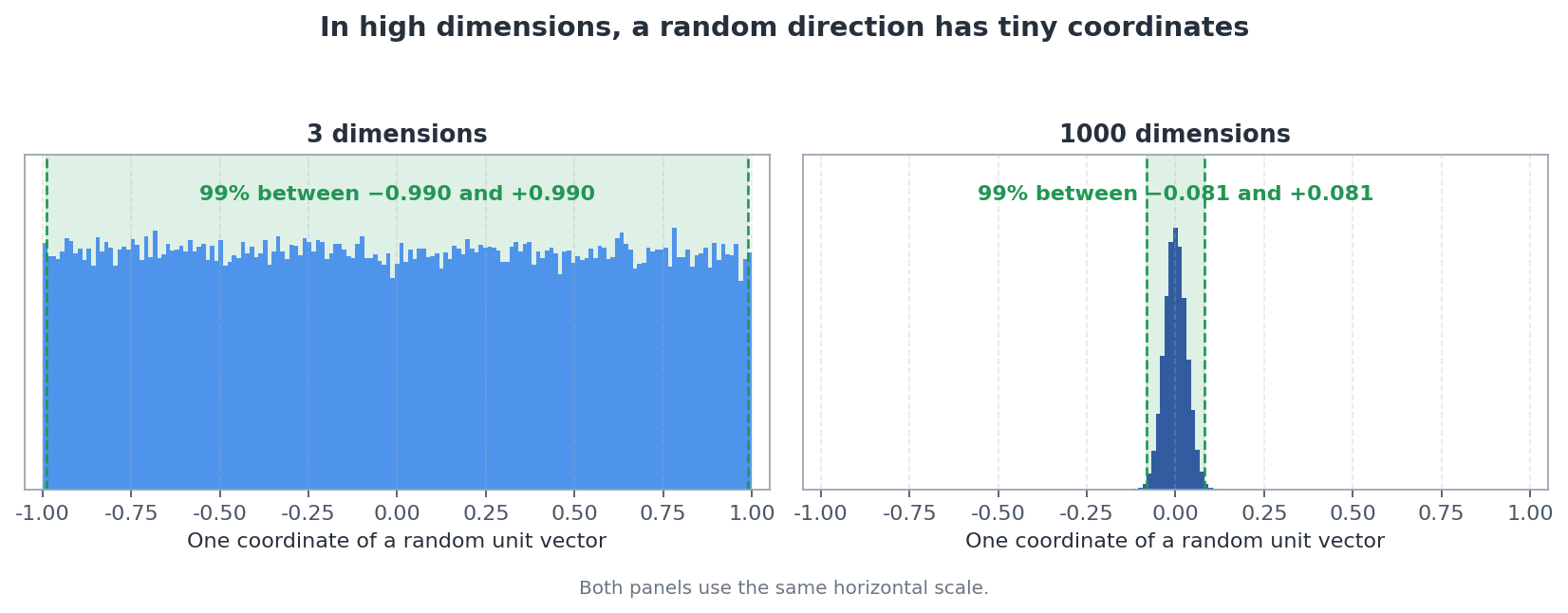
For example, a single coordinate of a random unit vector always lies in [−1, 1]. In three dimensions, its values span almost the entire interval; in 1000 dimensions, 99% of samples fall within ±0.081. Its typical magnitude is only on the order of 1/√D.
We can therefore approximate the orthogonal error term as zero to obtain the following unbiased estimator:
⟨o,q⟩ ≈ ⟨ō,q⟩ / ⟨ō,o⟩The numerator can be computed quickly at query time using bitwise operations and SIMD, while the denominator is a scalar stored for each data vector. A simplified view of its error bound is:
Error bound ∝ √((1-⟨ō,o⟩²)/⟨ō,o⟩²) × 1/√(D-1)This reveals two key properties of RaBitQ: higher dimensionality produces a more concentrated error range, and a quantized direction ō closer to the original direction o produces a smaller error bound. During search, this bound can be used to eliminate candidates that clearly cannot enter the Top-K.[1][4]
Extending from 1-bit to Multiple Bits
The original RaBitQ keeps only the sign of each coordinate. When higher precision is needed, Extended RaBitQ[2] adds extra bits, allowing more values per dimension and extending the codebook from the vertices of a hypercube to a regular grid. The unbiased estimator above relies on one key condition: every codeword in the codebook must be a unit vector. The grid points must therefore be normalized onto the unit sphere. The challenge is that the grid point nearest to the original vector is not necessarily the one whose direction is closest after normalization.[5]
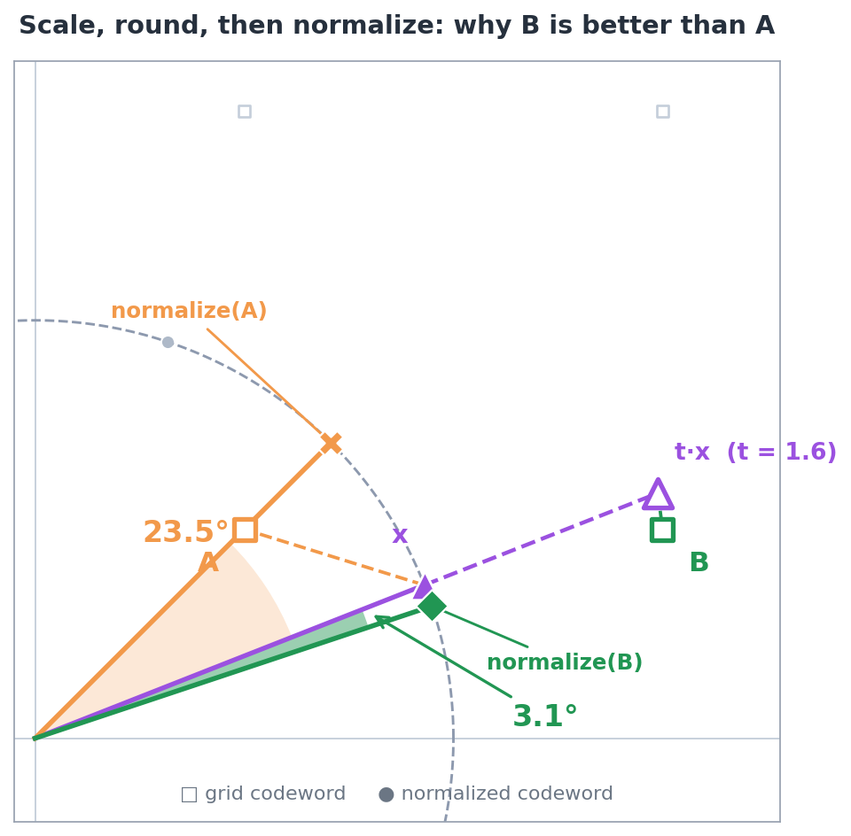
In the figure, rounding the coordinates of the original point x directly selects A, giving an angular error of 23.5° after normalization. Scaling x to t·x without changing its direction and then rounding the coordinates selects B, reducing the angular error to approximately 3.1°. Scaling preserves the target direction but changes the rounding result, making it possible to find a codeword closer to the original direction.
The value t=1.6 is only an example in the figure, not a fixed parameter. Extended RaBitQ tries multiple scaling factors for each vector, compares the resulting angular errors, and selects the codeword in the normalized codebook that is closest to the original direction. The authors prove that some scaling factor can always recover this optimal codeword[2][5]. The search for a scaling factor happens during construction. At query time, the inner product between the query vector and the quantized code can still be computed directly, without first decompressing it to FP32, using the same form of computation as scalar quantization.
RaBitQ thus covers 1-bit through multi-bit quantization within a single framework: 1-bit offers the highest compression, while extra bits progressively improve distance estimates.
How Zvec Implements RaBitQ
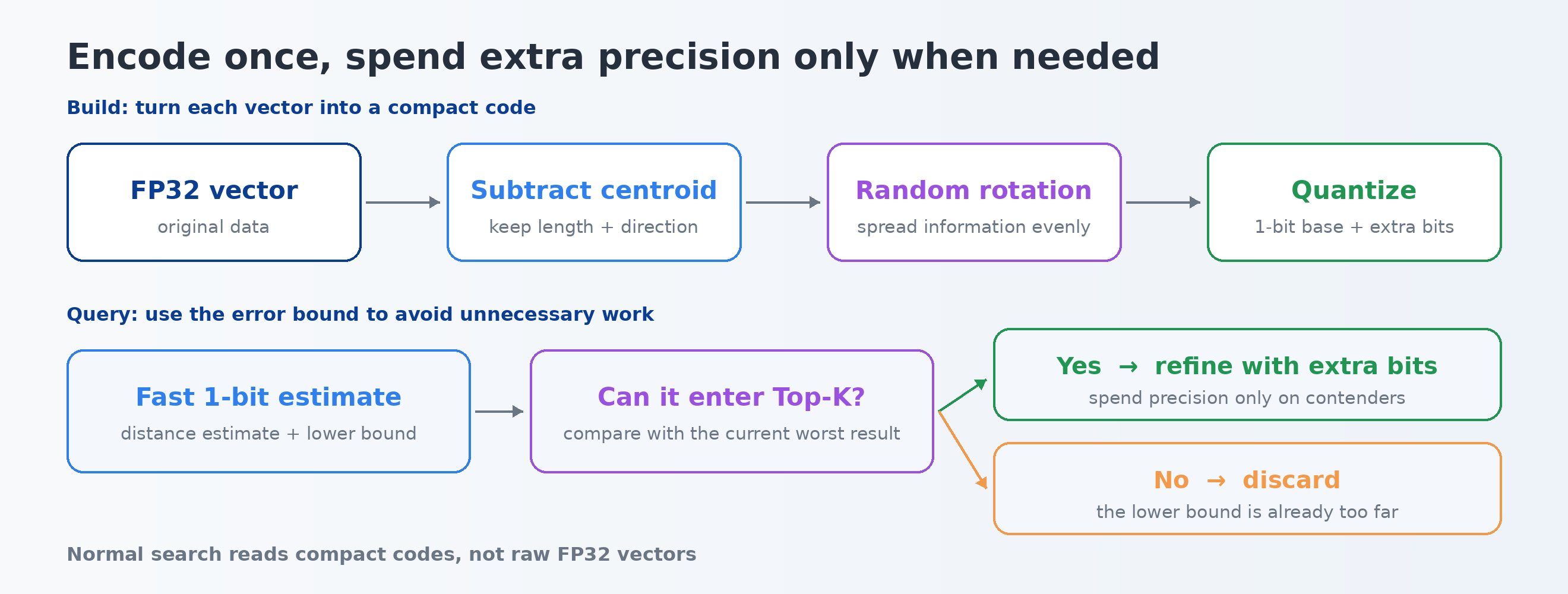
Random rotation. Zvec defaults to a Fast Hadamard Transform–based rotator (FHT Kac Rotator), applying a fixed four-round Kac walk to residual vectors with O(d log d) complexity. If the vector dimension is not a multiple of 64, the vector is zero-padded to align with the internal dimension.
Layered quantization. The base encoding retains only the sign bit of each coordinate, encoding positive values as 1 and negative values as 0. A d-dimensional FP32 vector thus becomes d bits. Zvec uses total_bits to control the total number of bits per dimension. The default is 7: 1 sign bit plus 6 additional bits. The additional bits are generated using the scale-and-round strategy described above, following the authors' extension[2] and the implementation in NTU's RaBitQ-Library[3].
Two-phase distance estimation. This is the most direct practical use of the error bound. Search does not perform a full quantized-distance computation for every candidate. Phase 1 uses SIMD to compute the inner product between the query vector and the candidate's binary code, producing both an estimate, est_dist, and a theoretical lower bound, low_dist. A candidate proceeds to Phase 2 for refinement with its extra-bit code only if low_dist is below the estimated distance at the top of the current Top-K heap. The error bound is therefore more than a theoretical result: it directly serves as a pruning condition.
Runtime SIMD dispatch. The Zvec team contributed runtime SIMD dispatch to the official RaBitQ-Library, allowing a single x86 binary to select AVX2 or AVX-512 automatically based on CPU capabilities. This makes precompiled binaries and Python wheels easier to distribute across different x86 environments[6].
Zvec's Two RaBitQ Indexes
RaBitQ answers the question of how to estimate distances quickly; the index structure determines where to look for candidates. Zvec offers two combinations: HNSW-RaBitQ searches along a nearest-neighbor graph for low-latency queries, while IVF-RaBitQ first selects inverted lists and then scans their codes in batches for high-throughput workloads.
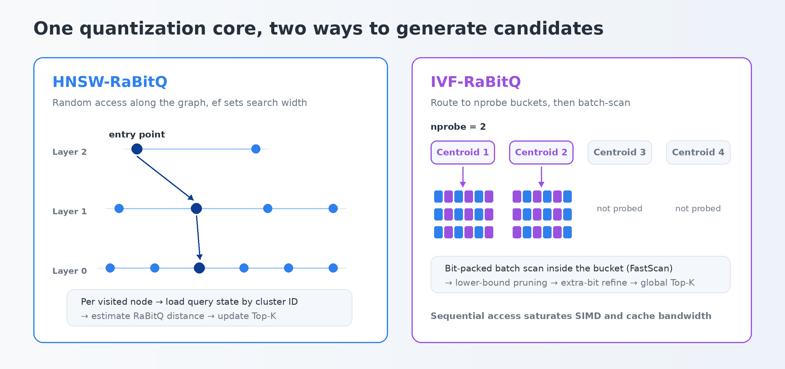
| Aspect | HNSW-RaBitQ | IVF-RaBitQ |
|---|---|---|
| Candidate generation | Hierarchical nearest-neighbor graph traversal | Centroid routing followed by inverted-list scanning |
| Query tuning parameter | ef | nprobe |
| Access pattern | Random access along the graph | Contiguous batch scans within each list |
| Typical focus | Online serving, low-latency queries | Batch retrieval, throughput-first workloads |
Both indexes require optimize() to build a persistent accelerated index. Before that, newly written data remains queryable through FLAT scans in in-memory segments. Run optimize() promptly after bulk writes.
In the implementation, HNSW-RaBitQ builds its graph using original FP32 distances and searches using quantized distances, so total_bits does not change the graph structure. IVF-RaBitQ stores codes within each list in transposed groups of 32, computes distances in batches with SIMD, and uses the error lower bound to reduce extra-bit computations.
Parameter Tuning
RaBitQ has no single parameter configuration that works for every dataset. Fix the dataset, Top-K, and target recall, then tune in the following order:
- Build the database with the default 7-bit quantization and construction parameters.
- Sweep
effor HNSW ornprobefor IVF to obtain a recall–QPS curve. - If space is a concern, test 4-bit or 1-bit quantization and repeat the query-parameter sweep.
- If the target recall is still out of reach, enable reranking with original vectors: tune
effor HNSW orscale_factorfor IVF.
| Parameter | Applicable indexes | Role |
|---|---|---|
total_bits | HNSW, IVF | Controls quantization bit width; fewer bits save space but generally increase distance-estimation error |
ef | HNSW | Controls the graph-search scope; larger values generally improve recall at a higher query cost |
nlist | IVF | Controls the number of inverted lists; choose based on dataset size and distribution |
nprobe | IVF | Controls the number of lists scanned per query; larger values generally improve recall and increase scanning work |
scale_factor | IVF | Takes effect only when reranking with original vectors; controls the number of candidates to rerank |
Conclusion
The core value of RaBitQ in Zvec is estimating distances directly from compact codes and using an analyzable error range to reduce unnecessary computation. HNSW-RaBitQ targets low-latency graph search, while IVF-RaBitQ targets batch scans of inverted lists. Both use total_bits to balance precision and space, and both support reranking with original vectors. Choose and tune them according to target recall and QPS, memory quota, and the available construction window.
Future work will focus on optimizing KMeans training and centroid quality, as well as supporting more CPU architectures and operating systems, to further improve construction speed, recall, and query efficiency.
Get Involved
Zvec is open source under the Apache 2.0 license. We welcome you to try it, share feedback, and contribute. If you obtain different results on your own data, please open an issue with the dataset characteristics, index parameters, and benchmark methodology.
- GitHub: https://github.com/alibaba/zvec
- Documentation: https://zvec.org
Appendix: Benchmark Details
Test Environment
The tests use an Alibaba Cloud ecs.g9i.4xlarge instance with 16 vCPUs and 64 GiB of memory, with swap disabled. Both the benchmark processes and the ES container are pinned to 8 physical cores; the 16-thread results represent SMT oversubscription. Zvec and Faiss are both built in Release mode with GCC 12.3.0 and use AVX-512.
The HNSW comparison uses Elasticsearch 8.18.8 with 1 shard, 0 replicas, _source disabled, a 4 GiB JVM heap, and a force-merge into a single segment. The IVF comparison uses Faiss IndexIVFRaBitQ. Internal OpenMP parallelism is fixed to a single thread on both sides, with concurrency provided by the benchmark driver.
| Dataset | Vectors | Dimensions | Distance | Queries |
|---|---|---|---|---|
| GIST-1M | 1,000,000 | 960 | L2 | 1000 |
| Cohere-1M | 1,000,000 | 768 | Cosine | 1000 |
HNSW: Reranking, Construction, and Concurrency Scaling
Zvec uses 1-bit codes to generate candidates quickly, then reads their original FP32 vectors for reranking. Elasticsearch BBQ has rescore_vector enabled.
With 8 threads at matched recall, Zvec delivers 11.0×–12.6× the throughput of ES on GIST and 5.9×–16.0× on Cohere. As recall approaches its upper limit, more candidates require reranking, and the throughput advantage gradually narrows. In additional tests with reranking disabled, ES reaches a lower maximum Recall@10 than Zvec: 0.321 vs 0.597 on GIST-1M and 0.750 vs 0.766 on Cohere-1M.
Construction time and index size are shown below:
| Dataset | Metric | Zvec 1-bit | Elasticsearch BBQ |
|---|---|---|---|
| GIST-1M | End-to-end database construction | 317.1 s | 963.2 s |
| GIST-1M | Complete index | 3.91 GiB | 4.46 GiB |
| Cohere-1M | End-to-end database construction | 345.3 s | 799.8 s |
| Cohere-1M | Complete index | 3.16 GiB | 4.72 GiB |
With 1-bit quantization, Zvec builds the database 3.04× as fast on GIST and 2.32× as fast on Cohere. Since both complete indexes retain the original FP32 vectors, their directory sizes do not achieve the theoretical compression ratio of the quantized codes alone. Zvec's 1-bit index is 12% smaller than ES on GIST and 33% smaller on Cohere.
Finally, concurrency scaling:
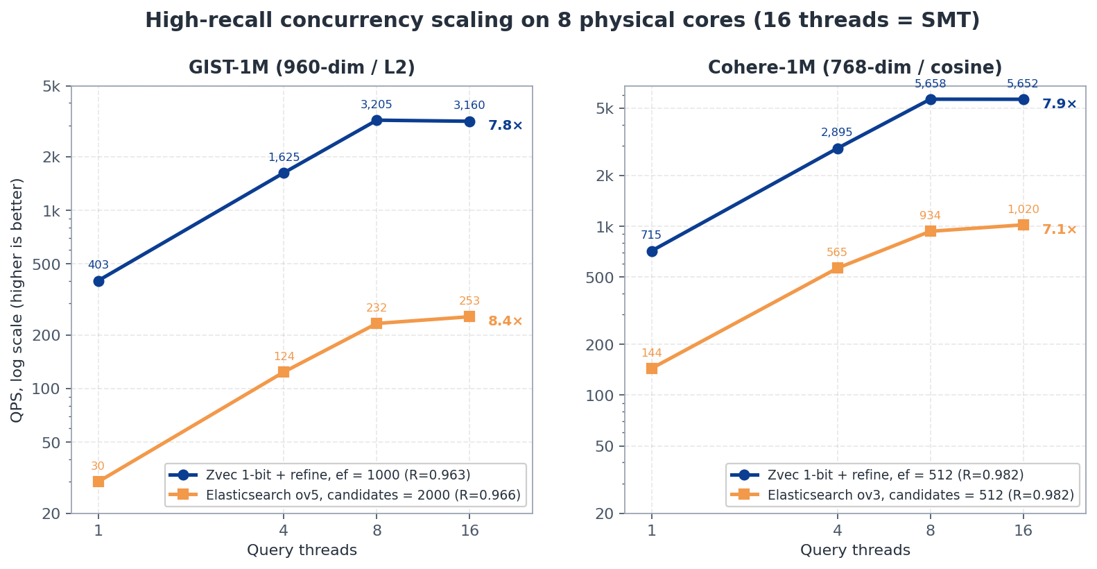
The figure uses high-accuracy configurations with approximately matched recall. When scaling from 1 to 8 threads, Zvec achieves 7.95× on GIST and 7.91× on Cohere, while ES achieves 7.73× and 6.49×, respectively. Both see limited gains once the thread count exceeds the number of physical cores.
IVF: Construction and Concurrency Scaling
Zvec's main disadvantage is in construction:
| Dataset | Zvec 7-bit | KMeans training portion | Faiss 7-bit | Time ratio |
|---|---|---|---|---|
| GIST-1M | 122.1 s | 108.2 s | 80.2 s | 1.52× as long |
| Cohere-1M | 89.0 s | 78.6 s | 85.2 s | 1.04× as long |
KMeans training accounts for roughly 90% of Zvec's 7-bit construction time. On GIST, Zvec takes 1.52× as long to build as Faiss. On Cohere, the two are close, with Zvec taking 1.04× as long. In terms of space, Zvec's 7-bit index is 6.5% smaller than Faiss on GIST and 24% smaller on Cohere.
For concurrency scaling:
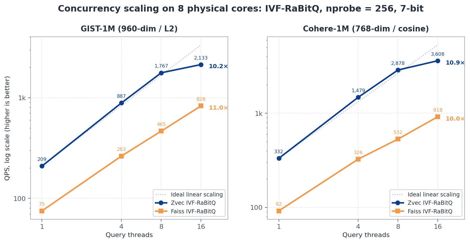
With nprobe=256 and 7-bit quantization, Zvec achieves 8.4×–8.7× scaling from 1 to 8 threads, compared with 5.8×–6.2× for Faiss. Both enter a region of diminishing returns once the thread count exceeds the number of physical cores.
References
[1] Jianyang Gao, Cheng Long. RaBitQ: Quantizing High-Dimensional Vectors with a Theoretical Error Bound for Approximate Nearest Neighbor Search. SIGMOD 2024.
[2] Jianyang Gao et al. Practical and Asymptotically Optimal Quantization of High-Dimensional Vectors in Euclidean Space for Approximate Nearest Neighbor Search.
[3] RaBitQ-Library, VectorDB-NTU.
[4] Jianyang Gao. Quantization in the Counterintuitive High-Dimensional Space. dev.to, 2024.
[5] Jianyang Gao. Extended RaBitQ: an Optimized Scalar Quantization Method. dev.to, 2024.