DiskANN: Scaling Vector Databases to Hundreds of Millions of Vectors
Abstract: Zvec's latest release introduces a native DiskANN index that stores raw vectors and the graph structure on SSD while keeping only a PQ-compressed "map" in memory. This cuts memory costs for hundred-million-scale workloads by an order of magnitude while preserving high recall. On the Cohere 1M dataset, Zvec DiskANN delivers 1.5x–2.4x higher single-threaded query throughput than Microsoft's open-source DiskANN at similar recall levels, with build times reduced by 36%–54% in our tests.
When Memory Can't Hold Hundreds of Millions of Vectors
Picture this: you're building an enterprise RAG system for a mid-size company. You need to index a decade's worth of contracts, support tickets, and meeting notes — roughly 230 million 768-dimensional vectors. If you go with HNSW, the most common choice for vector search, the FP32 raw data alone will consume nearly 650 GB of memory. Factor in the graph structure and runtime overhead, and even a 512 GB machine starts to struggle. And that's just to get the system running.
For datasets in the millions, HNSW is hard to beat — microsecond latency, dead simple. But once you cross the tens-of-millions threshold, memory cost becomes the elephant in the room.
DiskANN takes a straightforward approach: if it doesn't fit in memory, don't put it all in memory. Most of the data lives on SSD, with only a lightweight "compressed map" (a PQ codebook) staying in RAM. At query time, you consult the map to narrow down directions, then fetch the full-precision vectors from disk for final scoring. This reduces memory requirements for large-scale workloads by roughly an order of magnitude compared with in-memory HNSW, while preserving high recall. With modern NVMe drives routinely delivering 100K+ IOPS, that's a trade worth making. Here's a quick guide to picking the right index:
| Use Case | Index | Rationale |
|---|---|---|
| < 10M vectors, latency is king | HNSW | All in-memory, microsecond responses |
| 10M–100M+, cost-sensitive | DiskANN | Same recall, 10x less memory |
| Need 100% exact results | Flat | Brute-force search, zero information loss |
Zvec ships DiskANN as a first-class native index type. It shares the same Builder/Streamer/Reducer component model and the same Segment lifecycle as HNSW and IVF. For users, switching between DiskANN and HNSW is a matter of changing a single parameter at table creation time.
Getting Started
Creating a DiskANN index collection is as simple as swapping HnswIndexParam for DiskAnnIndexParam:
import zvec
from zvec import DataType, VectorSchema, MetricType, Query
from zvec import DiskAnnIndexParam, DiskAnnQueryParam

schema = zvec.CollectionSchema(
    name="massive_vectors",
    vectors=[
        VectorSchema(
            "embedding",
            DataType.VECTOR_FP32,
            dimension=768,
            index_param=DiskAnnIndexParam(
                metric_type=MetricType.COSINE,
                max_degree=64,
                list_size=100,
            ),
        ),
    ],
)

coll = zvec.create_and_open(path="./diskann_example", schema=schema)
At query time, a single list_size parameter controls the recall-vs-speed trade-off:
results = coll.query(
    queries=Query(
        field_name="embedding",
        vector=query_vector,
        param=DiskAnnQueryParam(list_size=200),
    ),
    topk=10,
)
Think of list_size as "how many extra steps you're willing to take" — a larger value explores more candidates via beam search, yielding higher recall at the cost of more disk I/O. In practice, a value between 100 and 300 is enough to hit 95%+ Recall@10; there's little reason to pay a steep price for those last few percentage points.
Performance: How Much Faster?
We benchmarked Zvec's DiskANN implementation against Microsoft's open-source DiskANN.
Test environment: Alibaba Cloud g9i 4xlarge (16 vCPU, 64 GiB, PL2 SSD / 100,000 IOPS).
Datasets: GIST — 1M vectors, 960 dimensions, Euclidean distance, 1,000 queries. Cohere — 1M vectors, 768 dimensions, cosine distance, 1,000 queries.
Note: Query benchmarks use a BFS cache of 10,000 nodes.
Build Speed
| Dataset | Zvec | MS DiskANN | Speedup |
|---|---|---|---|
| GIST | 14 min | 22 min | 1.55x |
| Cohere | 8 min | 17.5 min | 2.21x |
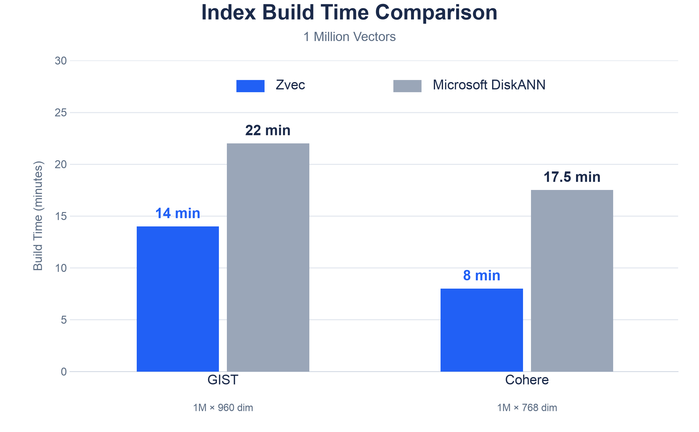
A series of engineering optimizations give Zvec roughly a 1.5x edge in build speed over Microsoft's DiskANN.
Build-Time Optimizations
-
Write directly to disk format — no second pass. Traditional DiskANN builds work in stages: first read the data to train PQ, then read it again to build the graph in memory, then re-read the in-memory graph node by node to pack it into sector-aligned disk format. Zvec short-circuits this pipeline: the in-memory graph layout is already the same layout the search path will read, so a single dump writes everything to disk. No intermediate re-read, no single-threaded re-sort, no temp file thrashing.
-
Contiguous memory for the graph, not per-node allocations. Zvec stores all node vectors and neighbor lists in one contiguous buffer — accessing a node is just a pointer offset, with zero extra allocation and great CPU cache behavior. Traditional approaches allocate a separate dynamic array per node; at hundred-million scale, that's hundreds of millions of tiny heap allocations that hammer the allocator and shatter cache locality.
-
Parallel PQ training + striped locks. During PQ training, each dimension chunk runs its own k-means independently (they're embarrassingly parallel, yet traditional implementations serialize them). During multi-threaded graph construction, Zvec uses a pool of 65,536 striped locks instead of one lock per node. The lock array costs only about 1 MB of memory, and the probability of two threads colliding on the same lock is just 1/65,536 — avoiding both the memory overhead of per-node locks at scale and the contention of coarse-grained locking.
Query Throughput
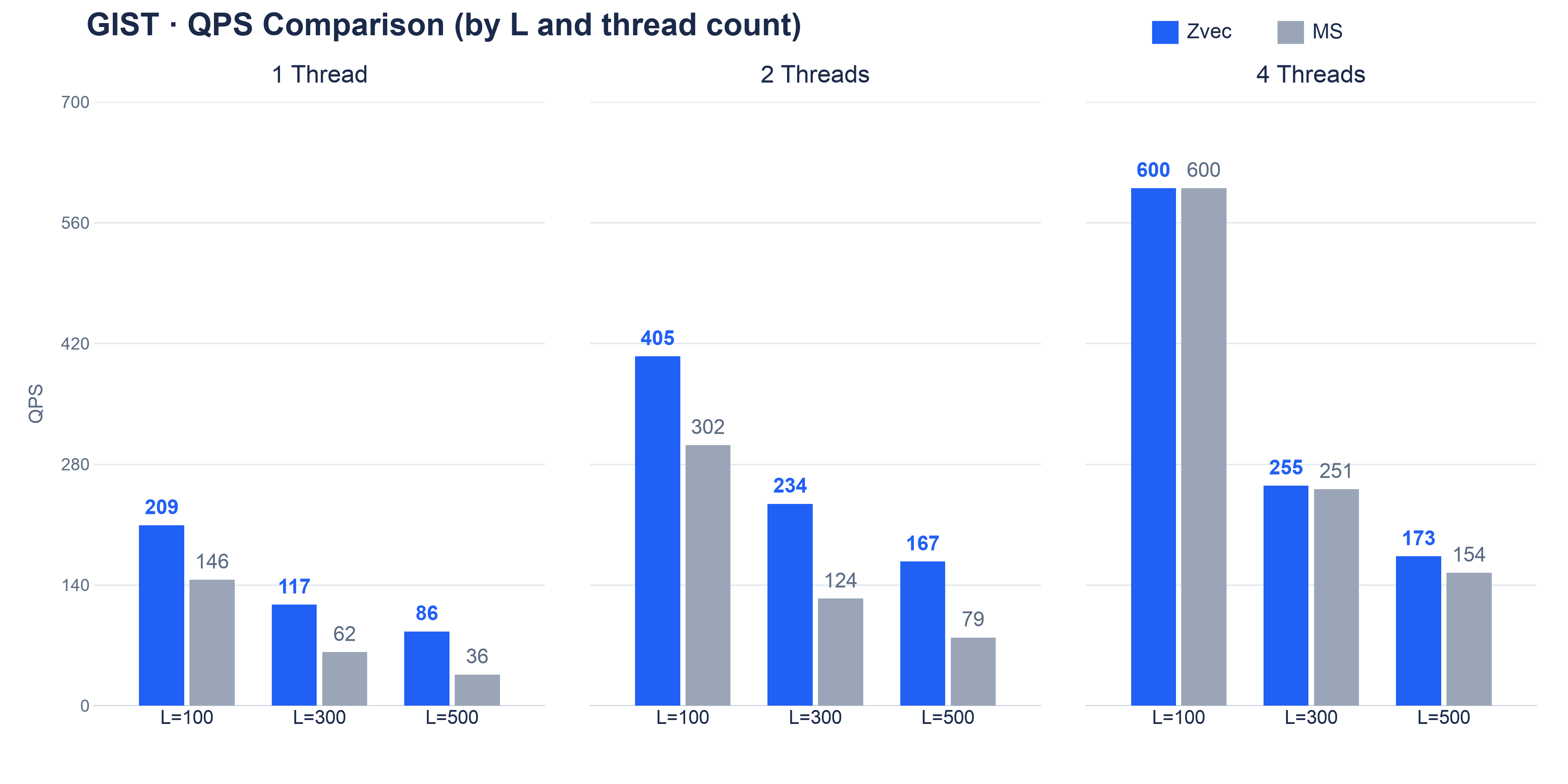
GIST dataset:
| Metric | Zvec L100 | Zvec L300 | Zvec L500 | MS L100 | MS L300 | MS L500 |
|---|---|---|---|---|---|---|
| Recall@1 (%) | 93.90 | 98.30 | 98.80 | 92.90 | 98.00 | 98.40 |
| Recall@10 (%) | 91.18 | 97.51 | 98.82 | 89.96 | 97.19 | 98.59 |
| Recall@50 (%) | 86.47 | 95.74 | 97.83 | 84.73 | 95.33 | 97.74 |
| QPS (1 thread) | 209.2 | 117.1 | 86.3 | 145.8 | 61.6 | 35.6 |
| QPS (2 threads) | 405.3 | 233.5 | 166.6 | 301.8 | 123.9 | 78.8 |
| QPS (4 threads) | 600.3 | 255.0 | 173.3 | 600.3 | 250.9 | 153.7 |
Cohere dataset:
| Metric | Zvec L100 | Zvec L300 | Zvec L500 | MS L100 | MS L300 | MS L500 |
|---|---|---|---|---|---|---|
| Recall@1 (%) | 98.20 | 99.40 | 99.60 | 97.80 | 99.50 | 99.60 |
| Recall@10 (%) | 98.30 | 99.49 | 99.67 | 98.09 | 99.54 | 99.71 |
| Recall@50 (%) | 96.45 | 99.09 | 99.53 | 95.87 | 99.06 | 99.53 |
| QPS (1 thread) | 238.2 | 142.9 | 94.3 | 158.9 | 65.5 | 40.0 |
| QPS (2 threads) | 493.6 | 270.8 | 184.3 | 325.5 | 129.5 | 81.6 |
| QPS (4 threads) | 618.5 | 267.5 | 179.1 | 630.2 | 252.8 | 160.8 |
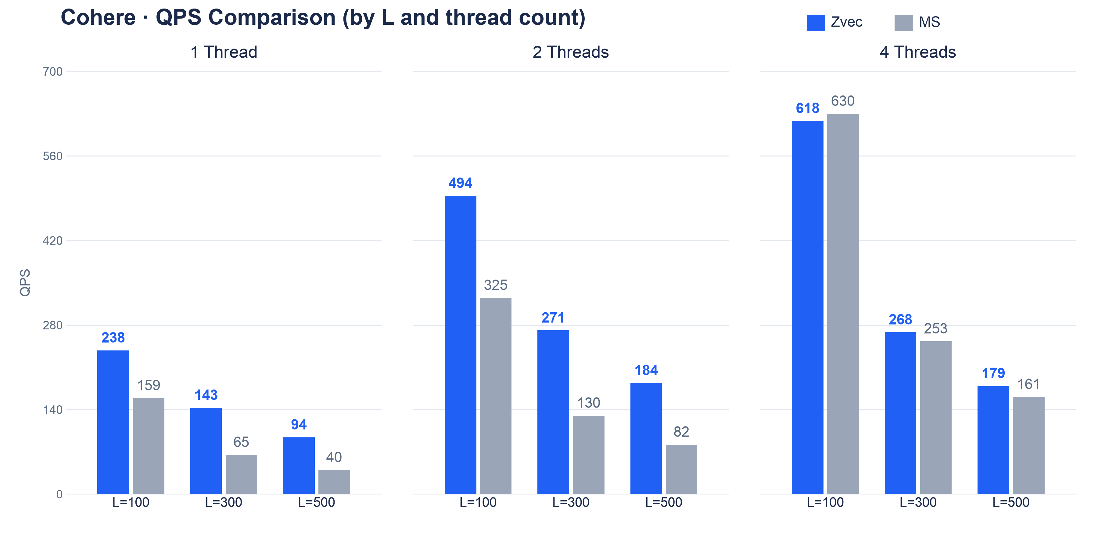
At L=300 — a sweet spot for production use — Zvec's single-threaded QPS approaches or even exceeds 2x that of Microsoft's DiskANN (1.9x on GIST, 2.2x on Cohere), and the gap widens as list_size grows (at L=500, both datasets show roughly 2.4x). Recall is essentially on par.
The throughput advantage narrows as thread count increases: at 4 threads under full load, both implementations are roughly comparable (0.98x–1.13x). The scaling curves tell the story: from 1 to 4 threads, Microsoft's DiskANN scales nearly linearly (~3.9x–4.3x), while Zvec achieves a more modest ~1.9x–2.9x. This isn't because Zvec "can't scale" — it's because the two implementations draw their performance from different sources. Zvec's single-thread lead comes from lower per-query latency (an async I/O pipeline that overlaps CPU and disk, plus a wider beam that reduces round trips), which means Zvec saturates the bandwidth of this PL2 SSD with just two or three threads. Microsoft's DiskANN has higher per-query latency but each thread spends more time idle. By 4 threads, both are bumping up against the disk's physical bandwidth ceiling.
Query-Time Optimizations
The throughput gains don't come from any single silver bullet — they're the result of optimizations stacked across multiple layers:
-
Asynchronous batch reads. Beam search doesn't read and process nodes one at a time. Instead, each round batches up all the nodes that need visiting, submits them in one shot via libaio, and then reaps results as they complete. Nodes that arrive first immediately go into distance computation while the remaining I/O is still in flight with the kernel. The CPU processes previously-fetched nodes in the gaps between disk returns, overlapping compute and I/O. By contrast, traditional DiskANN on Linux doesn't support true async — every hop blocks until the entire batch of I/O completes before the CPU can continue, leaving it spinning its wheels. The ability to genuinely overlap CPU and disk is the primary driver of the single-query latency gap.
-
O(1) "visited" marking. Graph traversal needs to ask "have I been to this node already?" at every step — tens of thousands of times per query on a hundred-million-node graph. The conventional approach uses a bitmap, but that requires a
memsetto zero it out at the start of every new query. Zvec uses a ByteMap instead: each node gets one byte that records "which query round last visited me." Starting a new query simply increments the round counter, invalidating all stale marks in O(1). A fullmemsetonly happens when the uint8 wraps around. Traditional implementations, by comparison, use a hash set to track visited nodes — every query pays hash-probe overhead for hundreds or thousands of lookups and insertions, then has to walk every bucket to clear the set when the query ends. -
Wide beam, fewer detours. Getting to the target means disk round trips on every hop — the fewer hops, the better. Zvec adaptively scales beam width up to 8–32 depending on search breadth; at L=300 it typically converges in about 10 hops. A narrow beam (default of 2 in traditional implementations, 8 in our tests) needs around 37 hops — three to four times more I/O round trips.
-
Distance computation that actually uses your CPU. Exact distance calculation sits on the hottest path and gets called relentlessly. Zvec dispatches at runtime to AVX-512, AVX2, SSE, or NEON based on what the CPU actually supports; on AVX-512-capable hardware, that's roughly 1.5x faster than an implementation hardcoded to AVX2. Traditional implementations ship a single AVX2 path and leave the rest of the silicon on the table.
-
Near-zero per-query overhead. Zvec gives each thread its own local context pool, with all buffers pre-allocated at load time. A new query just resets and reuses the buffer, copies in the query vector, and goes — zero lock contention. Traditional implementations check out a temporary workspace from a concurrent queue with a lock on every query and check it back in with another lock; at high call frequencies, that locking overhead adds up.
Peak Memory: Where the Savings Come From
Beyond throughput, DiskANN's other big advantage shows up in the memory comparison with HNSW (FP32, single-thread peak memory, MB):
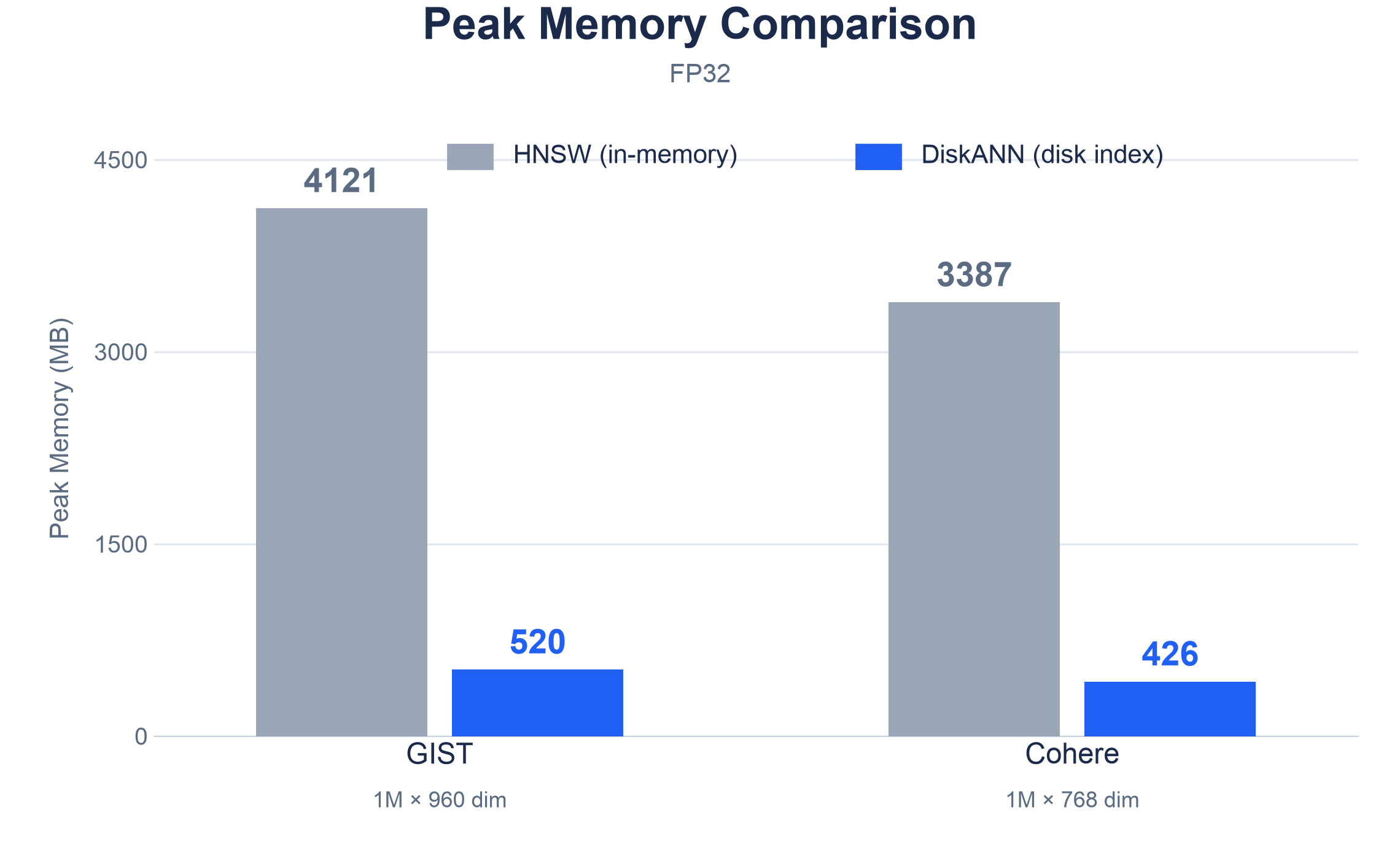
With the same FP32 data, HNSW consistently uses about 8x more memory than DiskANN. The reason is straightforward: HNSW keeps the full graph structure and all FP32 raw vectors in RAM (~4 GB for the 1M x 960-dim GIST dataset, ~3.4 GB for the 1M x 768-dim Cohere dataset). DiskANN, by contrast, only holds the PQ tables and a 1 MB access filter in memory.
Scale that 8x gap to a hundred-million-vector workload and HNSW needs hundreds of gigabytes of RAM, while DiskANN needs only tens of gigabytes.
Architecture: Making DiskANN Part of Zvec
Zvec's storage is built around Segments as the fundamental unit. When DiskANN was added, it plugged into the existing framework as a new index type following the standard Zvec contracts. This means DiskANN inherits Zvec's write, delete, export, recovery, and merge logic out of the box — no separate consistency handling needed for the disk-based index.
On-Disk Layout
The index file uses 4,096-byte sectors as its basic unit (aligned for O_DIRECT), with the following structure:
| Section | Contents |
|---|---|
| Meta | Header: document count, dimension, entry point, max degree, etc. (fits exactly in one 4 KB sector) |
| PQ Meta | PQ codebook: 256 cluster centroids, dimension partitioning scheme, global centroid |
| PQ Data | Compressed codes: each vector encoded as chunk_num bytes |
| Vector | Vector data: raw vectors followed by neighbor lists, nodes packed and sector-aligned |
| Key & EntryPoint | Primary key mapping and entry point list |
Each graph node on disk looks like this: [vector data | neighbor count | neighbor ID list | padding to sector boundary]. Small nodes can share a sector (avoiding waste); large nodes can span multiple sectors. The payoff is clean: reading a node is always one or a few whole-sector reads, going straight to the SSD via O_DIRECT, bypassing the page cache, with no extra memory copies.
How the Graph Is Built
Building a DiskANN index proceeds in four steps:
- Train the PQ codebook: Randomly sample 200K vectors, subtract the global mean, partition by dimension chunks, and run k-means independently on each chunk to produce 256 cluster centroids per chunk.
- Build the Vamana graph: For each node, find a high-quality set of neighbors via greedy search — this is the most compute-intensive step.
- Prune: Trim nodes that exceed
max_degreeback down. - PQ encoding: Use the codebook to compress each vector into a sequence of bytes.
The second step is where the magic happens. For each new node, Vamana does two things:
-
Find candidates (greedy search): Start from the entry point (the medoid — the vector closest to the centroid of all vectors) and progressively approach the target. At each step, jump to the closest unexplored neighbor in sight until no closer option remains, yielding a set of points nearest to the target.
-
Filter neighbors (RobustPrune): This is what sets Vamana apart from a plain greedy graph. Instead of taking the K nearest neighbors, it demands directional diversity among neighbors — think of it like choosing signposts at a crossroads: if two signs point in nearly the same direction, you only keep one. Concretely, if candidate B's direction is already "blocked" by an already-selected neighbor A (i.e., A is closer to B than the current node is), B gets skipped. The strictness is controlled by the parameter α=1.2. The result is a graph that covers more directions with fewer edges, leading to fewer hops at search time.
-
Back edges: After selecting neighbors, a reverse edge is added back from each selected neighbor. If this pushes a neighbor's degree above 1.3x max_degree, it gets pruned again. This avoids dead ends where you can get from A to B but not from B to A.
The locking strategy for multi-threaded construction is also carefully tuned: 65,536 mutexes form a striped lock pool, with the lower 16 bits of each node ID used as a hash. Different nodes almost always land on different locks (collision rate: 1/65,536), so there's no need to allocate a lock per node (at hundred-million scale, the locks themselves become a memory burden), nor do threads queue up behind coarse-grained locks.
Why PQ Training Parallelizes
The traditional approach slices, say, 768 dimensions into several chunks and runs k-means on each chunk sequentially. But the clustering on each chunk is completely independent — chunk 1's centroids have nothing to do with chunk 2's. Zvec's MultiChunkCluster simply assigns each chunk to a different thread and trains them in parallel, each running to convergence independently. When dimensions are high and chunk counts are large (768 dimensions default to 384 chunks), the parallel speedup is substantial.
Search: What Happens Inside a Query
A single DiskANN query unfolds in three phases:
-
Phase 1: Prepare the "map" When a query arrives, the system computes the distance from the query vector to every PQ cluster centroid, producing a lookup table of shape
[chunk_num x 256]— this is the "map" for all subsequent routing. Estimating the PQ distance to any node after this is just a matter of looking up a few values in the table and adding them together. -
Phase 2: Beam Search Starting from the entry point, the system maintains a candidate queue sorted by PQ distance, sized at
list_size. Each iteration pops the most promising candidate from the front of the queue: if it's in cache, it reads straight from memory; if not, the sector offsets are batched up and submitted as a single async I/O request.
Once a node's data arrives, two things happen: the exact distance is computed using the full vector and inserted into the top-k heap (the source of final results), and the PQ map is used to estimate distances to all of the node's neighbors, feeding promising ones back into the candidate queue. This loop continues until no candidate in the queue looks more promising than the worst result currently in the top-k.
The core trade-off: PQ distances steer, exact distances judge. PQ lookups and additions are blazing fast but noisy — they make sure no good candidate is missed. Exact distances require disk I/O but guarantee result quality.
-
Phase 3: Cache as a safety net The first two or three hops from the entry point follow nearly the same path every time (the entry point and its immediate neighbors). These nodes are cached in memory via BFS at index load time. A cache hit means beam search starts with almost zero disk I/O, which makes a noticeable difference in p99 latency.
-
Engineering details
- FP16 support. A C++ template unifies the interface across FP32 and FP16. FP16 halves each vector's on-disk footprint and halves the data read per I/O. In testing, Recall@10 dropped by just 0.16 percentage points (from 99.49 to 99.33) — for most use cases, that's essentially free storage savings.
- Compile-time dispatch for the access filter. The traditional approach uses virtual functions to switch between BloomFilter, BitMap, and ByteMap. But in graph traversal this function gets called tens of thousands of times per search, and the indirect jump through a vtable prevents the compiler from inlining. Zvec uses macro expansion for static dispatch at compile time, letting the compiler inline the calls completely and eliminate per-invocation overhead.
- Observable performance metrics. Every query automatically reports: total time broken down into I/O wait and CPU compute, disk pages read, distance computations performed, cache hit rate, and graph traversal hops. When latency spikes, comparing
io_ustocpu_usimmediately tells you whether to add caching or optimize the distance function. - Dynamic I/O backend framework. At runtime, Zvec automatically probes and selects the most suitable I/O backend for the current environment, with graceful fallback for compatibility. For libaio, a dedicated framework handles dynamic detection and
dlopen-based loading.
Parameter Tuning Cheat Sheet
| Parameter | Purpose | Default | Tuning |
|---|---|---|---|
| max_degree | Max edges per node | 64 | Higher → better recall, larger nodes, more I/O |
| list_size (build) | Search width during build | 100 | Higher → better graph quality, slower build |
| list_size (search) | Beam width at query time | 200 | Higher → better recall, more disk I/O |
| cache_node_num | Number of hot nodes to cache | 0 | Set to 1–10% of total; immediate latency win |
A practical starting point: max_degree=64, cache_node_num at 5% of total vectors, and list_size starting at 100 and working upward — watch the recall-QPS curve to find the sweet spot your workload can live with.
Summary
The core idea behind Zvec DiskANN boils down to this: make disk-based graph search a native capability of the vector database, and use a compressed map to scale to hundreds of millions of vectors.
For users, the change is simple:
- Write
DiskAnnIndexParamat table creation, and hundred-million-scale workloads drop from near-TB memory to single-digit GB. - Tune
list_sizeat query time — one knob for the recall-latency trade-off. - Share the same API as HNSW and IVF — switching index types is a one-line config change.
- Enable FP16 to halve storage again, with virtually no recall loss.
Under the hood, it's the combined effect of Vamana graph construction, parallel multi-chunk PQ training, 4K sector-aligned layout, BFS-level caching, and ByteMap O(1) clearing that delivers "higher throughput at the same recall, with an order of magnitude less memory."
HNSW is the right call when memory is plentiful and latency is paramount. DiskANN is the right call when scale is massive and cost matters. The two complement each other, giving users a choice that maps cleanly to their real-world constraints.
What's Next
The current release ships end-to-end on Linux (x86_64) with libaio. The roadmap includes expanding I/O backends and platform coverage:
- io_uring backend: Adopt io_uring on newer kernels as the default async I/O path, replacing libaio.
- Windows: Wire up IOCP as the async I/O backend so DiskANN can deliver strong throughput on Windows.
- macOS (Darwin): Adapt kqueue-based async disk reads so developers can run, debug, and benchmark DiskANN natively on Mac.
- ARM: Cover ARM servers (e.g., Yitian, Graviton) and beyond.
- Mobile: Adapt to the memory-constrained environments of iOS and Android for on-device vector search.
Stay tuned!
Zvec is open-source under the Apache 2.0 License. We welcome you to try it out, share feedback, and contribute.
- GitHub: https://github.com/alibaba/zvec
- Docs: https://zvec.org